
An incoming inspection plan is used to decide whether or not to accept a batch, based on samples taken from the batch. Several types of sampling are taken into account when drawing up an inspection plan:
- Control by attributes (single, double, progressive planes)
- Measurement control (method S, s, progressive).
The module IQC (Incoming Quality Control) Ellistat's IQC module not only calculates standardized inspection plans, but can also be used to create customized inspection plans, which are often much more suitable than standardized plans. Even the highly innovative progressive measurement method. It should be noted that this method, with constant efficiency, enables sample sizes to be reduced considerably.
Control plan for receiving attributes
For this type of incoming inspection, each part is measured according to an OK/KO scale. The batch is accepted if the number of KOs measured is below a certain limit.
Receipt control for attributes can be :
- Simple: a certain number of parts are measured once. Acceptance of the batch is defined at the end of the measurement of all the parts.
- Double: a first batch of parts is measured. The batch is accepted if the number of defects is less than "Acceptance 1". The batch is rejected if the number of defects is greater than "Reject 1". Otherwise, a second batch of parts is measured and the batch is accepted if the number of defects is less than "Acceptance 2". Rejected otherwise. This type of incoming inspection limits the number of parts measured.
- Progressive: batch acceptance or rejection is calculated for each measurement. This type of control is the most efficient. > Find out more
Advantages of attribute-based control: easy to set up
Disadvantages of attribute reception control AQL below 1% cannot be achieved without significantly increasing the number of parts measured.
Control plan reception of measurements
For this type of incoming inspection, each part is measured on a quantitative scale. The batch is accepted if the mean of the batch is more than k standard deviations from the nearest tolerance (k or k factor being defined by the incoming inspection).
The incoming inspection can be :
- Simple: a certain number of parts are measured once, and acceptance of the batch is defined at the end of the measurement of all the parts,
- Progressive: batch acceptance or rejection is calculated for each measurement. This type of control is the most efficient.
Advantage of measurement-receipt inspection: significantly reduces the number of parts measured compared with attribute inspection.
Disadvantage of control by measurement: Each part must be measured quantitatively.
Efficiency curve
When setting up a statistical incoming inspection, you need to be aware that it's not possible to stop 100% incoming defects.
Supplier and customer must therefore agree on an acceptable level of quality, i.e. the average percentage of defects that the incoming inspection must allow to pass.
The control efficiency curve is designed to predict control results as a function of the batch quality rate measured.
Take the following example:
We receive a batch of 1000 parts containing 50 defects. The incoming inspection is as follows. 80 parts in the batch are inspected. The batch is accepted if 1 defect or less is measured. Otherwise, the batch is rejected. According to the laws of descriptive statistics, we can show that (open descriptive/discontinuous statistics) :
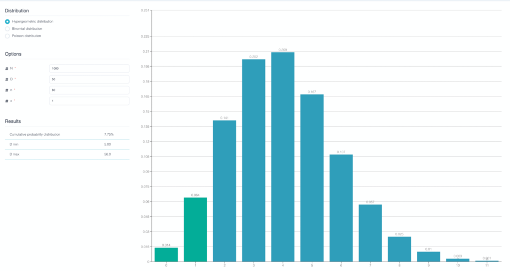
The probability of measuring 1 defect or less is 7.7%. Consequently, this batch has a 7.7% chance of being accepted and a 92.7% chance of being rejected.
We can therefore predict that with an inspection of 80 parts and an acceptance level of 1 defect, a batch of 1000 parts containing 5% of defects has a 7.7% chance of being accepted.
The efficiency curve is therefore used to give the acceptance probability for all possible batches. The x-axis of the efficiency curve is the percentage of defect contained in the batch. The Y axis is the acceptance percentage.
The following figure shows the efficiency curve for an inspection of 80 parts and an acceptance level of 1 defect:
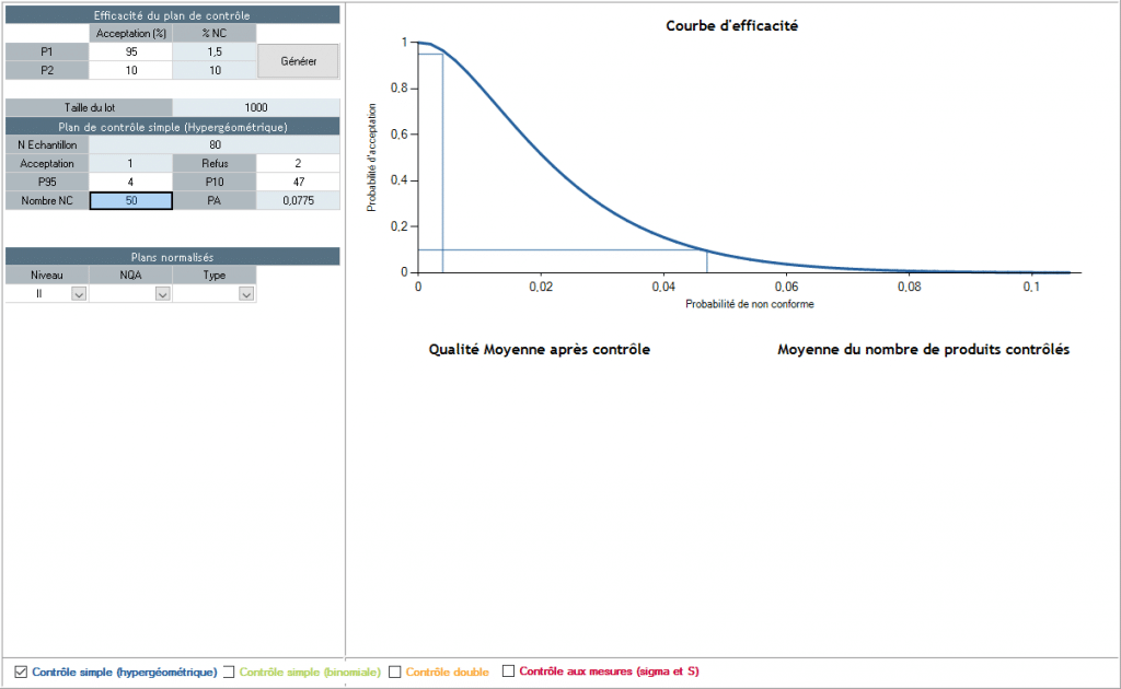
We can see that if there are 50 defects, the acceptance level is 7.7%.
P95 and P10
To characterize this curve, we generally use two characteristic points of the curve:
P95 The P95 corresponds to the rate of defects in a batch resulting in an acceptance level of 95% with the control in place. In the previous example, the P95 is 4, i.e. a batch containing 4 defects has a 95% chance of being accepted.
P10 The P10 corresponds to the rate of defects in a batch resulting in an acceptance level of 10% with the control in place. In the previous example, the P10 is 47, i.e. a batch containing 47 defects has a 10% chance of being accepted.
