To explain the central limit theorem, let's take this as our starting point. God doesn't play dice," once said A.Einstein about quantum mechanics, calling into question one of the foundations of modern physics. However, experiments carried out in the 20th century proved him wrong, and it is now accepted that all observables in this world govern according to distribution probabilities and are subject to Heisenberg's uncertainty principle. The world is random...
Understanding random phenomena is fundamental to understanding how the world works. A central theorem of statistical data analysis can be demonstrated mathematically: the central limit theorem.
Any system resulting from the sum of many factors, independent of each other and of an equivalent order of magnitude, generates a distribution law that tends towards a normal distribution.
This theorem shows the importance of the normal distribution in analyzing the variability of an observable. To illustrate this, let's roll a die 1000 times in succession and observe the distribution of results:

The distribution follows a uniform distribution, i.e. the die is equally likely to land on 1, 2, 3, 4, 5 or 6. The distribution does not resemble a normal distribution.
Let's roll 10 dice 1000 times in a row and observe the distribution of the results of the sum of these 10 dice:
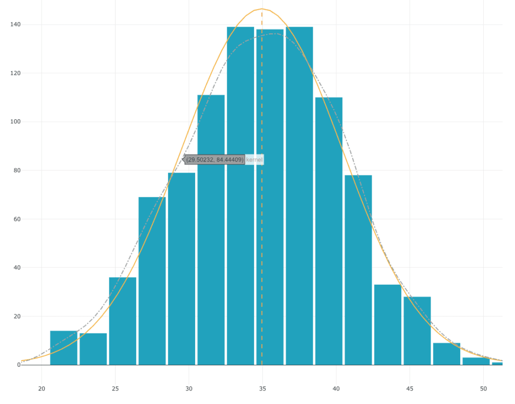
Although each of the dice follows a uniform distribution, the distribution of the sum of the 10 dice follows a bell curve. This distribution is very close to a normal distribution.
Indeed, if we follow the central limit theorem :
- We have a system
- Resulting from the sum of many factors (here the sum of 10 dice)
- Independent of each other (the result of one die has no influence on the result of another die)
- The order of magnitude of each of the dice is equivalent
The distribution generated by this system tends towards a normal distribution. All in all, it's quite intuitive. When 10 dice are rolled, there is only one combination that will produce a result of 10 (all the dice landed on 1), whereas there are thousands of combinations that will produce a result of 35. As a result, outcomes close to 35 are much more likely to occur than extreme outcomes such as 10 or 60. The distribution law obtained is therefore close to a normal distribution law.
The systems we usually observe have this type of distribution, because they satisfy the assumptions of the central limit theorem. Let's take the example of machining a part:
- It's a system that produces a feature.
- The deviation of the characteristic from the target results from the sum of many factors (vibration, material hardness, tool positioning error, etc. ....).
- The factors are independent of each other (machine vibration has no influence on material hardness).
- The order of magnitude of these deviations is equivalent to
The distribution of parts therefore tends towards a normal distribution, which is what we observe when we measure a series of parts.