In this article, we'll look at how to calculate the various capability indices, in particular Cp, Pp and Ppk.
To fully appreciate the capability of a process, the notion of time is particularly important, as two types of variability can be distinguished:
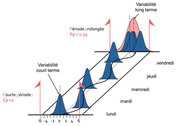
- Short-term variability: when two parts are produced consecutively, these two parts will not be completely equivalent due to intrinsic machine variations. This short-term variability depends mainly on the machine.
- Long-term variability: when you produce on the same process over a longer period of time, the machine itself will go out of adjustment, and series changes, material batch changes, etc. will bring new sources of variation. This long-term variability depends not only on the machine itself, but also on numerous external sources of variability, and on the way in which the process is managed.
Example
To illustrate this point, let's look at the following production diagram:

Production for the week is the result of production on the different days of the week. However, as the diagram above illustrates, production conditions on different days of the week are not equivalent. The centering of the process is not the same between production on Monday, Tuesday, etc...
As a result, we can see that the variability over the whole week (red curve) is greater than the variability observed over a short period of time, as it takes into account fewer phenomena that can cause variability, such as a setting or a change of material.
There are therefore two ways of characterizing process capability, depending on the type of variability observed: short-term cp and long-term pp.
Short-term Capability Index Cp
Short-term CpShort-term capability: Short-term capability characterizes the process's ability to produce good parts, taking into account only the process's intrinsic variability (the variability between two consecutive parts). Short-term capability is denoted Cp and is calculated by :
Cp= \frac{\text{tolerance interval}}{6*\text{short term dispersion}}= \frac{\text{tolerance interval}}{6*\sigma_{\text{short term}}}
In general, we want :
Cp > 2
Long-term capability index Pp
Long-term PpLong-term capability: Long-term capability characterizes the ability of the process to produce good parts over a long period of time, i.e. taking into account adjustments and process modifications that may occur. Long-term capability is denoted Pp and is calculated by :
Pp=\frac{tolerance interval}{6∗long term dispersion}=\frac{tolerance interval}{6∗σ_{long term}}
In general, we want :
Pp > 1.33
Since long-term capability takes into account more sources of variability than short-term capability, we necessarily have :
\text{long term dispersion} < \text{short term dispersion}
And so
Pp < Cp
If this is not the case, this does not mean that short-term dispersion is greater than long-term dispersion, but that dispersion is not stable over time.
Methods for calculating capability indices Cp, Pp, Ppk
As we've just seen, Cp and Pp are calculated using the same formula. Cp and Pp are differentiated by the time periods over which variability is calculated. There are several methods for calculating Cp and Pp.
Method 1: Taking several samples at regular intervals
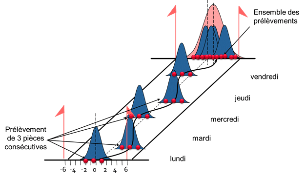
The first method for calculating short- and long-term variability is to take several samples at regular intervals.

Short-term variability : Short-term variability is calculated using the intra-series standard deviation of all samples:
\sigma_{\text{short term}}=\sigma_{\text{intra sample}}
Long-term variability : 50 parts are sampled over a characteristic period of the process, to take into account multiple sources of process variation such as adjustments, tool changes, material changes, etc. Long-term variability is calculated by :
\sigma_{\text{long term}}=\sigma_{\text{all sample}}=\sqrt{\sum_{}^{}(\frac{^{(x_{i}-\mu)^{2}}}{n-1})}
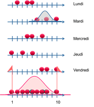
Example: The following sample is taken

The tolerance interval is [1 ;10].
We calculate the intra-series standard deviation :
\sigma_{\text{short term}}=\sigma_{\text{intra sample}}=1.7321
The standard deviation of all parts is calculated:
\sigma_{\text{long term}}=\sigma_{\text{all sample}}=\sqrt{\sum_{}^{}(\frac{^{(x_{i}-\mu)^{2}}}{n-1})}=2.6904
We therefore deduce :
Cp= \frac{\text{tolerance interval}}{6*\text{short term dispersion}}= \frac{\text{tolerance interval}}{6*\sigma_{\text{short term}}= \frac{9}{6*1.7321}=0.87
Pp=\frac{\text{tolerance interval}}{6*\text{long term dispersion}}= \frac{\text{tolerance interval}}{6*\sigma_{\text{long term}}=\frac{9}{6*2.6904}=0.56
Ppk=\frac{Min(\text{tolerance max}-\mu,mu-\text{tolerance min})}{3*\text{long term dispersion}}= \frac{4.33}{3*2.6904}=0.54
Method 2: By taking two separate samples
The second method for calculating short- and long-term variability is to take two separate samples.
- Short-term variability: 50 consecutive unadjusted parts are taken to calculate the short-term variability of the process. Short-term variability is calculated by :
\sigma_{\text{short term}}=\sigma_{\text{all sample}}=\sqrt{\sum_{}^{}(\frac{^{(x_{i}-\mu)^{2}}}{n-1})}
- Long-term variability: 50 parts are sampled over a characteristic period of the process, to take into account multiple sources of process variation such as adjustments, tool changes, material changes, etc. Long-term variability is calculated by :
\sigma_{\text{long term}}=\sigma_{\text{all sample}}=\sqrt{\sum_{}^{}(\frac{^{(x_{i}-\mu)^{2}}}{n-1})}

