To test normality, there are several tests that can be used to validate or invalidate the hypothesis that the distribution of parts follows a normal distribution. The tests most commonly used are :
- The Chi2 test
- The Anderson-Darling test
Normality test with Chi2 test
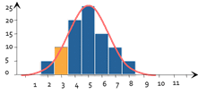
To check the normality of a distribution, our first intuition would be to plot the histogram of the distribution of observed variables. Then, to compare whether this histogram more or less resembles the Gauss curve usual.

That's exactly what the Chi2 test is all about. It adds to this intuition a small dose of statistical calculation. The principle is as follows:

d_i=\frac{(N_i-NP_i)^{2}}{NP_i}
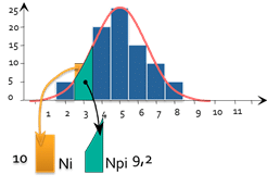
For each bar of the histogram, we can calculate :
- Ni : Number of pieces actually observed (here 10)
- Npi: Number of pieces theoretically observed if the distribution were normal (here 9.2)
- di represents the "number of misplaced parts".
We then calculate
D=\sum_{}^{}D_i
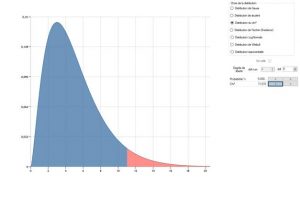
and it turns out that D follows a distribution law with n-2 degrees of freedom (N being the number of classes). We can then calculate the probability of obtaining such a value.

For example, for a histogram with 7 classes, if we have calculated a D of 11.07, we calculate that there are 5% to obtain such a value or more if the distribution law of the parts is indeed normal.
The result of the test will therefore be 5% and we generally conclude as follows:
- If X < 5%: the distribution of the variables is not considered to follow a normal distribution.
- If X >= 5%: the normality hypothesis is accepted, and the distribution can be considered to follow a normal distribution.
What to do in case of non-normality
The central limit theorem tells us:
Any system, resulting from the sum of many factors independent of each other and of an equivalent order of magnitude, generates a distribution law that tends towards a normal distribution.
But we can also reason in the opposite way. If we observe a non-normal distribution, then one of the theorem's hypotheses is invalid:
- Case 1: the system is not the sum of many factors: it may be the product of many factors or other. In this case, the distribution law may be different, and in general a transformation (taking the log of the result, for example) will restore a normal distribution.
- Case 2: The factors are not independent of each other
- Case 3: The factors are not of the same order of magnitude :
- One factor outweighs the others. In this case, we need to find the factor in question, as it alone generates a significant source of variability.
- An outlier is polluting the distribution. In this case, we need to find the cause of the outlier and eliminate it if the cause can be explained.
In both cases, it is not necessary to find a distribution law corresponding to the observed variability. In fact, this distribution law will not be repeatable over time, as it is due to a single parameter, and will therefore have no predictive properties.
If the origin of the non-normality is due to case 1, it's time to find the corresponding distribution law, especially if you want to predict the percentage of values outside tolerance. To do this, you can use the suggested distribution laws at the bottom of the window in Data Analysis module to see if one of the distributions can account for the observed data:

