


Optimizing a formulation is not the same as optimizing a process, for a geometric reason: the proportions of the components total of 100 %. You cannot increase the resin content without reducing something else, and a standard design of experiments that assumes independent factors does not apply.
This module covers all the fundamentals of Bayesian optimization—Gaussian processes, explained proposals, convergence, leave-one-out diagnostics, strategies, noise, search quality, and demo mode—by applying them to the simple, the domain of valid combinations.
1. The Components
Each component has a name, a minimum and a maximum as a fraction, and perhaps locked to a fixed value. The module continuously checks the feasibility For the set as a whole: terminals whose minimum values sum to more than 1, or whose maximum values sum to less than 1, do not define any feasible mix, and the program flags this before performing any calculations.
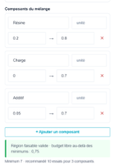
The initial plan is not an Audze-Eglais but a plan Maximin on the simplex : mixtures that are as far apart as possible within the permitted range. The module recommends a number of tests based on the number of components—at least seven, with ten recommended for three components—and sets an upper limit of 100.
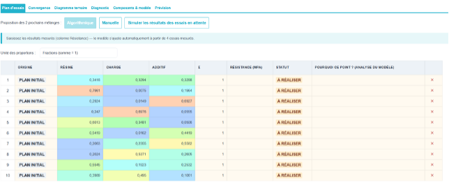
As data is entered, each test result is checked for missing values, non-numeric values, out-of-range values, or a sum other than 1. A command corrects invalid tests by resizing them to fit within the domain.
2. The ternary diagram
With three or more components, the dedicated tab displays a ternary diagram : the simplex triangle, the predicted answer highlighted in color, the tests conducted, the suggestions, and the areas unfeasible excluded by the bounds. A checkbox switches the display to show the uncertainty. If there are more than three components, the others are fixed at a single value, as shown on the Bayesian optimization map.
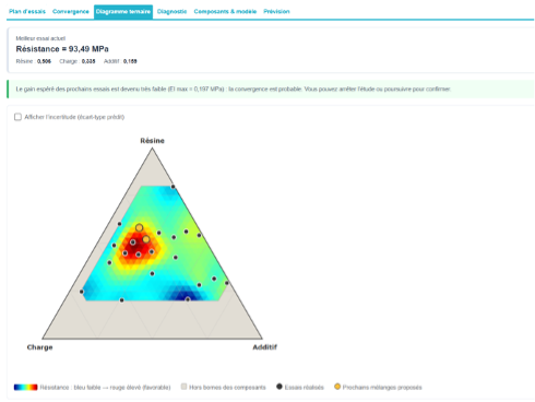
💡 The ternary diagram is the A representation of a mixture, and it’s worth learning how to read it: each vertex represents a pure component, each edge represents a binary mixture, and the center represents a mixture in equal parts. The areas shaded by the boundaries immediately reveal how much leeway the formulation constraints actually leave you—often less than one might imagine.
The remaining tabs—Test Plan, Convergence, Diagnostics, Factors & Model, and Forecast—are explained exactly as in Section 4, including the answers and suggestions.
The other tabs are the same as those for Bayesian optimization.