


This page includes four common calculations—without any datasets—that help ensure compliance with acceptance testing standards. ISO 2859 and 3951 and for calculating confidence intervals and making predictions ISO 16269-6 and ISO 16269-8.
1. IQC – Attributes
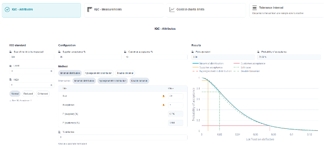
The acceptance inspection answers a simple question: Based on a sample, should the lot be accepted or rejected? This page covers both scenarios: finding a standardized checklist or creating a custom checklist.
1. Find a standardized chart (ISO 2859)
- Enter the lot size, the inspection level (I, II, or III—II by default; special levels S-1 through S-4 for costly or destructive inspections), and the AQL (acceptable quality level).
- You choose the type of withdrawal (single, double, or multiple) and the schedule: normal, increased after a series of refusals, or reduced when the history is good.
- The output includes: the code letter, the sample size n, and the acceptance criterion Ac and rejection criterion Re. This is exactly the row one would look up in the tables of the standard, with no risk of misreading.
2. Create a Custom Plan
- Either we directly specify n and Ac, and the software plots the corresponding efficiency curve: we can then see what this design actually allows.
- Either we start with the desired result: two points on the curve—a quality level we wish to accept almost always (p1, with supplier risk α) and a quality level we wish to reject almost always (p2, with customer risk β)—and the plan (n, Ac) is derived from them.
- This second approach is the most straightforward: it requires stating both the benefits and the risks, whereas a standardized plan assumes them implicitly.
💡 The efficiency curve is the true result, not the (n, Ac) pair. It gives, for each proportion of defective items in the lot, the probability of accepting it. Two plans with the same AQL can have very different curves: it is the sample size, not the AQL, that determines the power of discrimination.
⚠️ The NQA is not a quality objective, and a sampling plan does not guarantee the quality of an accepted lot: it merely limits, on average and across a series of lots, the probability of accepting a defective lot. A plan with Ac = 0 is also not the most stringent under all circumstances; it severely penalizes acceptable lots without improving the detection of clearly defective lots. Compare the curves before selecting this plan.
2. IQC – Measurements
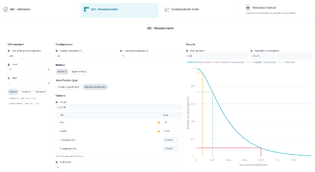
The same acceptance logic applies, but the decision is no longer based on a count of defective parts: it uses the measured value. For the same level of protection, a measurement-based plan requires far fewer parts than an attribute-based plan—which is its main advantage when inspection is time-consuming or costly.
1. Find a standardized map (ISO 3951)
- The input parameters are the same as those for the attributes: lot size, inspection level, AQN, and standard/enhanced/reduced inspection regime. In addition, the nature of the tolerance (unilateral or bilateral) and whether or not the process standard deviation is known must be specified.
- «Unknown sigma» method (s-method): The standard deviation is estimated based on the sample. This is the most common approach; it requires a slightly larger sample.
- «Known sigma» method (σ method): A standard deviation value is established and kept constant. The sample size is smaller, but the hypothesis must be tested regularly.
- Output: the sample size n and the acceptance constant k. The lot is accepted if the mean remains more than k standard deviations outside the tolerance limit—(Max. Tol. − X̄) / s ≥ k—and similarly on the lower side. For a two-sided tolerance, the decision is based on estimating the proportion of items outside the total tolerance.
2. Create a Custom Plan
- Either we specify n and k, and the efficiency curve shows what this plan actually allows.
- Either we specify two points on the curve—the quality level that should almost always be accepted (p1, supplier risk α) and the one that should almost always be rejected (p2, customer risk β)—and the pair (n, k) is derived from them.
💡 Comparing the two pages for the same case is the most telling exercise: for the same level of protection, the measurement-based plan often reduces the sample size by a factor of three or four. This is the argument to make when the test is destructive.
⚠️ This approach comes at a cost: the control plan assumes that the characteristic is normal. For an asymmetric or truncated distribution—such as a defect in shape, eccentricity, or a feature that has already been sorted—the estimated proportion outside tolerance is incorrect, and the control plan does not provide the promised protection. Verify that the distribution is appropriate before selecting a measurement plan; if in doubt, revert to attributes.
⚠️ One inspection plan per characteristic. Unlike attributes—where a part is either defective or not—dimensional inspection evaluates one dimension at a time: multiple critical characteristics require multiple inspection plans, and the overall risk of acceptance is no longer that of a single inspection plan.
3. Control Chart Limits
Plot an efficiency curve based on the parameters to determine the size of a circuit board before implementing it.
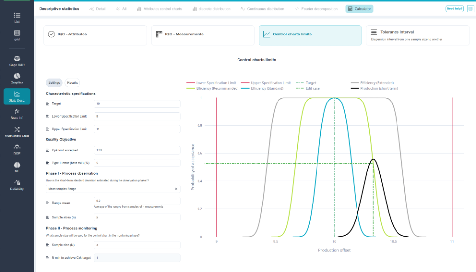
The calculation is performed in three steps: estimate the short-term sigma, choose the criterion for setting the limits, and then consult the efficiency curve to verify what the card, sized in this way, is actually capable of detecting.
1. The Origin of Short-Term Sigma
- Based on a set of measurements: intra-sample standard deviation (S̄/c4) or mean range (R̄/d2). This is the most reliable source, but it requires properly defined rational subgroups.
- Based on a known capability: σct = IT / (6 × Cp). Useful for sizing when only the process capability is documented.
- Fixed sigma: a historical or reference value, used when the map needs to remain comparable from one period to the next rather than being recalibrated for each batch.
⚠️ Short-term sigma determines everything else. When estimated using poorly constructed samples, it is inflated: the limits become too wide, and the map no longer detects anything. When estimated using too few samples, it is unstable, and the efficiency curve immediately reflects this.
2. The three sets of limits offered
| Limitations | Principle | A question they answer |
| ± 3 sigma (standard) | X̄ ± 3 σct / √n. These values depend only on the process dispersion, never on the tolerance. False alarm risk of approximately 0.27 %. | Has the process changed compared to itself? That is the criterion for stability. |
| Ensuring a minimum Cpk with a certain level of risk β | Limits derived from tolerances: LCI = Min. Tol. + 3 × Min. Cpk × σct + uβ × σct / √n, and similarly for the LCS. The term uβ × σct / √n accounts for the sampling uncertainty on the mean; β is the risk of falsely accepting a process whose actual Cpk is below the required value. | Does production still meet the required quality standards? That is the compliance criterion. |
| Interim Status | A middle ground between the two previous approaches: we maintain statistical sensitivity to change without requiring a response as long as compliance is not at risk. | Compromise: when neither stability alone nor conformity alone is enough to make a decision. |
💡 The choice isn’t about the accuracy of the calculation but about what you want to control. In a highly capable process, the limits guaranteeing a Cpk are significantly wider than ±3 sigma: we allow the mean to drift as long as compliance is not at risk, and we eliminate unnecessary interventions. In a just-capable process, on the other hand, the limits are tighter than ±3 sigma, and if they overlap, no adjustment will allow the tolerance to be maintained: the problem is dispersion, not control.
💡 The efficiency curve shows, for each possible offset, the probability that the map will detect it. This curve determines the sample size: doubling n narrows the limits to √n and flattens the curve, at the expense of sampling cost.
4. Dispersion Interval
The interval that contains a given proportion of the population, based on a sample size. It is calculated by Method S or Sigma Method.
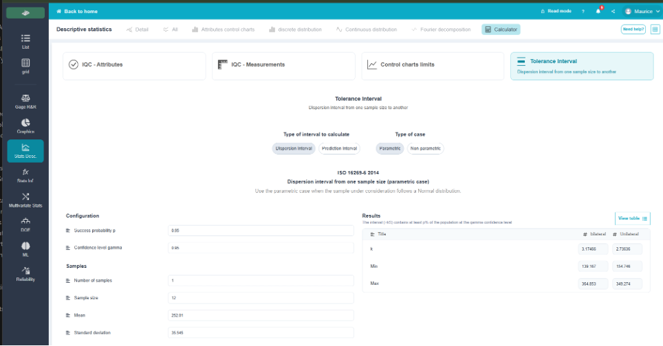
Based on a sample, we want to estimate not the mean but the population itself: within what range does a given proportion of the items fall, and with what level of confidence? This is the purpose of statistical dispersion intervals (ISO 16269-6) and prediction intervals (ISO 16269-8).
1. What We Understand
- The sample size n, the observed mean and standard deviation, or directly the parameters assumed in the a priori design.
- The proportion of the population to be covered (often 95 %, 99 %, or 99.73 %) and the associated confidence level (often 95 %).
- The type of interval: bilateral, or unilateral when only one boundary is relevant—a minimum resistance or a maximum concentration.
2. S Method or Sigma Method
- Method S: The standard deviation is estimated from the sample. The coefficient k then incorporates two uncertainties—one regarding the mean and one regarding the variance; the smaller n is, the larger k becomes. This is the general case.
- Sigma Method: The standard deviation is assumed to be known, based on historical data from a controlled process. The interval is significantly narrower, but it is valid only if this value is truly known.
- The limits are expressed as X̄ ± k × s (or k × σ), where the coefficient k is determined by calculation based on n, the target proportion, the confidence level, and the chosen distribution.
3. Three intervals that should not be confused
- Confidence interval: provides a range for a parameter, such as the mean or standard deviation. It narrows toward zero as n increases.
- Confidence interval (or statistical tolerance interval): encompasses a proportion of the population. It converges toward the true population interval, not toward zero.
- Prediction interval: provides a range for the next observation(s). This is the right tool for asking, «Will the next part produced fall within this range?».
💡 The most common use is to verify compliance in small production runs: if the 99% % / 95% % dispersion interval remains within the tolerances, we can state, with the specified confidence level, that the production meets the specifications. This is a more robust approach than a simple min-max comparison of the sample, which proves nothing about what has not been measured.
⚠️ The coefficient k is not 3: to cover 99.73% of the population with a 95% confidence level, k is significantly greater than 3 for a small sample, and only approaches 3 when n is large. Using X̄ ± 3s based on 20 measurements amounts to making a claim that the data does not support.
⚠️ Like the capabilities, these intervals assume a normal distribution by default. For non-normal data, check the fit or use the adjusted distribution rather than applying a normal k-value to a distribution that is not normal.
💡 The confidence interval is the tool you use when you ask, «I have 30 observations; what bounds can I guarantee for the population?» The answer depends heavily on the sample size, and the difference between 30 and 100 observations is often surprising.
5. Prediction Interval
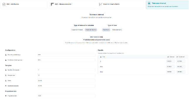
The prediction interval does not refer to a parameter or to the entire population; rather, it sets bounds for future observations. The question becomes, «Given what I have measured, between what limits will the next observation—or the next m observations—fall with a given level of confidence?».
1. What We Understand
- The results of the initial sample: sample size n, mean, standard deviation, or the reference standard deviation if the process is known.
- The number of future observations to be covered: one, or m future values.
- The level of confidence and the form—whether bilateral or unilateral.
- At the output, the terminals X̄ ± k × s. For a future observation with an estimated standard deviation, k = t(1−α/2; n−1) × √(1 + 1/n): the term 1 accounts for the variability of the upcoming sample, and the term 1/n accounts for the uncertainty in the mean.
2. When to Use It
- Qualification and testing: ensuring the quality of the next part, batch, or test based on a limited series.
- Monitoring: While an isolated measurement may have limited value if the process has not changed, a value outside the prediction interval is a signal, not a nonconformity.
- Focusing on a future shipment rather than on the inventory already produced: this is where confusion with the confidence interval proves most costly.
💡 A prediction interval is always wider than a confidence interval for the mean, and it does not narrow toward zero: even with an infinite number of measurements, the future part retains its own variability. Increasing n improves our understanding of the process, not the reproducibility of the next part.
💡 Covering future observations simultaneously widens the range: requiring that all 10 upcoming pieces fall within it is much more restrictive than requiring it for just one. The number of observations to be covered must therefore correspond to the actual commitment made.
⚠️ The calculation assumes that the process remains in the same state and follows a normal distribution by default. It does not predict anything following a change in settings, material, or tool: the interval covers observed variability, not future drift. The control chart remains the safeguard.