


Sequential bifurcation / dichotomous plans. When faced with a defect that could have many possible causes, we cannot afford to test each factor individually. Dichotomous screening eliminates most of them in just a few trials by grouping factors together rather than testing them one by one.
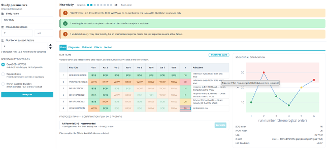
The principle: each factor is set to its own level the most favorable at first glance (BOB, Best of the Best) or the most unfavorable at first glance (WOW, Worst of the Worst). We construct a small number of configurations in which the suspected factors shift from one group to another, much like looking up a name in a dictionary by halving the stack of pages each time. An active factor gives itself away through the behavior of the group to which it belongs; an inactive factor blends into the group and disappears from the investigation.
💡 This is a method for identifying causes, similar to BOB vs. WOW and Component Inversion: it does not confirm a model, but rather narrows down a long list of suspects to a few likely culprits. The classic design of experiments then takes over to quantify and confirm the results.
1. How many trials, and why?
For N factors, N columns are open, but only k = ⌈log₂N⌉ Tests are required: 3 tests are sufficient for up to 8 factors, 4 tests for up to 16, and 5 for up to 24. Each factor is assigned a binary signature unique—its BOB or WOW position in each of the k trials—and no two factors ever share the same signature. It is this signature that makes it possible, once the trials are complete, to determine which of the grouped factors caused the response to change.
Before starting the tests, you must decide how the variation observed at each stage will be evaluated. There are three options to choose from in the left panel:
| Mode | Principle | When to Use It |
| Difference (BOB − WOW) / 3 | The dispersion is derived from the deviation itself; no repetition is necessary. | Rapid roughing; no dispersion data available. No significance test is possible in this mode: the conclusion remains qualitative. |
| Repeated Tests | Each configuration is measured several times; the standard deviation is estimated based on these repeated measurements. | Unknown dispersion, but the tests are inexpensive to repeat. |
| Known standard deviation | Enter a pre-determined sigma value—machine capability, gage R&R, SPC control chart. | The process is already under statistical control, and its residual sigma is documented. |
⚠️ In Repeated Trials mode, a single trial is not sufficient to estimate a standard deviation: at least two trials per configuration are required.
💡 The labels «BOB» and «WOW» are generic. The first two rows of the test table, as well as the name of each factor, can be edited: rename them using your workshop’s terminology (for example, «New» / «Worn,» «Supplier A» / «Supplier B»). Once customized, these labels will appear in the table cells instead of the words BOB/WOW.
2. Runs Tab: Review the tests
The central table shows, for each test, the setting for each factor (using its custom label) and a column Reading where to enter the measured value. A graph remains visible at all times next to the table, with the BOB and WOW bands positioned at ± your dispersion threshold: a value that falls within a band classifies the test, while a value between the two bands leaves it undecided (INC).
After each read, a status bar summarizes the status of the survey and immediately flags any anomalies: non-significant deviations, overlapping bands, or inconsistencies in the eliminations.
- A value within the BOB range confirms the BOB group for this test; ;
- A value within the WOW band confirms the WOW group; ;
- A value between the two bands is undecided : It does not yet allow us to rule out the factors in this trial, but that does not mean it is a lost cause (see the parsimony-based effect estimate)
3. Diagnostics Tab: The Elimination Trace
This is where the roughing-out process becomes verifiable. For each test, Ellistat displays which factors were eliminated (deemed inactive) and which ones remain suspects, along with the rationale behind each decision. A binary signature matrix records, factor by factor, its position in each trial, which makes it possible to understand in retrospect why one factor survived and another did not.
4. Multi-Vari tab: View survivors
A nested multivariate plot includes all surviving factors, sorted by decreasing effect size. It allows you to see at a glance whether one or two factors clearly dominate the others, or whether the effect is distributed among several factors of comparable importance—useful information for determining whether the study is complete or needs to be expanded.
5. Complete the confirmation plan
When multiple factors survive (m ≥ 2), the k screening tests are not sufficient to distinguish their individual effects: they are still confounded. Ellistat then suggests the additional tests needed to obtain an analyzable L4/L8 design with resolution III or IV, depending on the number of surviving factors. by reusing tests that have already been conducted, never starting from scratch.
| Survivors (m) | Proposed Plan |
| 1 | No additional information: the factor has been isolated; proceed directly to confirmation. |
| 2 to 4 | Supplement to a full factorial design or an IV solution, depending on the exact number of survivors. |
| 5 to 7 | Additional requirements for an L8 Resolution III (minimum) or IV. |
| 8 | A full factorial design or a fractional factorial design (Resolution IV) is required, depending on the interactions to be accounted for. |
6. Effects tab
The principle. Each factor in a dichotomous analysis has only two levels: BOB and WOW. Testing whether a factor has a significant effect on the response therefore amounts to testing whether the regression coefficient associated with this factor, in a linear model, is not zero.
Read the table. For each selected factor, the Effects tab displays:
| Column | Meaning |
| Effect | The mail carrier (with his personalized name). |
| Coefficient | Half of the difference between the BOB level and the WOW level in the response—the effect of the factor. |
| Standard Error | The uncertainty regarding this coefficient, given the completed plan. |
| T | The ratio of the coefficient to the standard error: this is the statistic for Student's t-test. |
| P | The associated p-value—to be interpreted in the same way as in §2: significant below 0.05, borderline between 0.05 and 0.1. |
| Significance | The verdict in a nutshell: significant or borderline. |
| VIF | Variance Inflation Factor. Measures the extent to which this factor is correlated with the others in the designed experiment. A high VIF indicates that the experiment is not balanced enough to properly isolate this factor—an additional confirmatory test may be necessary. |
At the bottom of the painting: the R² and the Adjusted R² (the proportion of the variation in the response explained by the model), and the constant (the predicted mean value when all factors are at their reference levels).
⚠️ The p-values in this tab are optimistic. The model displayed was not specified in advance: the factors listed here are those that survived the preliminary screening step based on an initial review of the data. This choice, made after the fact, artificially inflates the confidence suggested by the following p-values. They remain useful for comparing factors with one another, but should not be interpreted as the p-value of a test planned in advance; this is why Ellistat includes this warning directly on the tab.
The tab remains locked until the confirmation plan described in §8.5 is complete: with only one survivor (m = 1), there is nothing to resolve, and a specific message indicates this.
7. Method tab: Specify the method
This tab places dichotomous research in its methodological context and distinguishes between two very different historical contributions, although they are often conflated:
- the sequential branching (sequential bifurcation), developed by Bettonvil in his 1990 dissertation based on an idea by Jacoby and Harrison (1962), which groups factors into fixed bands centered around a reference standard deviation; ;
- the dichotomous plans, developed specifically to take advantage of the odd columns in the Taguchi tables and validate each cut-off point using an actual statistical test rather than a fixed range—z-test, Dixon test, and then t-test as more data are collected.
💡 The name «dichotomous search» chosen for this module is therefore not merely a simplification of terminology: it is the very term used in the French research that led to the development of dichotomous search algorithms.