


Multivariate analysis of variance compares cross-factors : Each setting on one corresponds to each setting on the other. On nested factors, the spindle belongs to one and only one machine, the workpiece to one spindle, the impression to one mold, and the position to one furnace; this model is not appropriate. The source of variation is the framework of these structures: it attributes the observed variability to each level of the hierarchy, from the coarsest to the finest.
It is also the only tool for observing the menu: there is nothing to trigger, nothing to exchange, nothing to filter. We make use of the variability that has already been generated and recorded by the process.
💡 Crossed factors → multivariate. Nested factors → sources of variation. If you select the wrong screen, Ellistat detects it and displays a button that switches to the other screen while keeping your selection.
1. Selection and Detection of the Structure
The selection follows the multivariate model: one quantitative Y variable and one or more qualitative X variables. You do not specify the hierarchy; Ellistat infers it from the data. A factor B is nested within a factor A if each of its levels appears only with a single level of A. If this relationship completely orders the selected factors, the structure is a pure hierarchy, and the calculation is initiated.
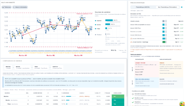
The breadcrumb trail for the Variance Components block displays the structure used in the example: Machine ▸ Pin ▸Part ▸ Runs, with, for each level, the number of modes and the number of modes per mode at the higher level: 3 machines, 12 spindles (4 per machine), 60 parts (5 per spindle), and 2 measurements per part. It cannot be modified: there is only one correct breakdown for a given hierarchy.
Below the thread, a sentence explains how the structure was deduced. In particular, it notes the reuse of the same names across different carriers: the «B1» pin on two different machines counts as two separate pins. If, on the other hand, these names refer to a common setting, the factors are crossed, and the multivari method must be used.
There is no choice of method, no fixed or random cells, and no model settings: all levels are treated as random—a batch, a pin, and a mold are samples of modalities, not exhaustive settings—and each level is tested against the one immediately below it. The components are estimated using restricted maximum likelihood (REML), as noted below the table; in a balanced design, REML coincides exactly with the expected mean squares used by the Gage R&R.
2. The conclusion is clear
The blue box summarizes the analysis in three sentences derived from the results. The first sentence contextualizes the variability in relation to a pivotal level: «82.8 % of the variability occurs above »Pièce’ in the equipment, not in the operation from one modality to another.” ” This is the guiding statement: it indicates whether the focus is on equipment or on control.”.
The second method identifies the dominant levels but refuses to designate a winner when their confidence intervals overlap: with 3 machines and 12 pins, Machine (50.4 %) and Pin (32.3 %) cannot be distinguished. Adjusting the hardware is warranted; determining which of the two levels is the true culprit would require further investigation. This caution is intentional—it is the screen’s primary function.
The third column shows the repeatability of the measurement and, if the characteristic has tolerances, the coverage of the tolerance interval by 6σ, as well as Pp and Ppk.
3. The two graphs
The nested multivariate plot uses the same graph you're familiar with, but the order of the factors is determined by the hierarchy: the data points are grouped by machine, then by spindle within each machine. The “Tolerances” and “Individual Values” buttons display the tolerance limits and the complete scatter plot of the measurements.
On the right, the Pareto chart of sources shows the proportion of variance accounted for by each level, including the residual. The thin line beneath each bar represents the 95 % confidence interval for that proportion: a line extending up to 100 % indicates that the displayed proportion is a rough estimate, not an exact measure. The «Proportion Explained by Hierarchy Levels» indicator (94.5 % in the example) is the complement of the residual: it is the fraction of the variability that your factors explain.
4. The table of variance components
Each line represents a level in the hierarchy, with the last level being the residual—the repetitions of the measurement at the finest level of detail. Nested levels are indented and labeled «in Machine» and «in Spindle.».
| Column | What She Says |
| DDL, Mean Square | Degrees of freedom and mean square error. |
| F, P-value | F is the ratio of the mean square of the level to that of the level immediately below it; the p-value is derived from this. The residual is not tested. |
| σ | Standard deviation caused by this source, in the unit of Y. |
| % variance | Proportion of the total variance attributable to the source. This column adds up exactly to 100 %. |
| IC 95 % | Confidence interval for this proportion. An interval that extends to 100 % indicates a level with too few observations to be estimated accurately. |
| % from IT | 6σ of the source relative to the tolerance range. Blank if the characteristic has no tolerances. |
| Conclusion | Test verdict — Yes, Very, No — using the guide's standard color-coding system. |
⚠️ The % values for IT are calculated using a quadrature method: they are not added together. Adding up this column results in a total greater than the actual tolerance consumption; this is not a calculation error.
5. PPK Simulation
This block does not appear only if the feature has tolerances. It answers the question, «What would I gain if I removed this source?» For each level, Ellistat Subtract the corresponding component from the total variance and recalculate Pp and Ppk using the observed mean. Also included are the «Rework to Target» row and the best source + rework combination. The rows are sorted by increasing gain, with the current situation at the top, and a marker at the threshold of 1.33.
Two important notes regarding the interpretation of the data, as noted below the table. Eliminating measurement repeatability does not improve the parts; it corrects the estimate. This line tells you what your actual Ppk is, excluding measurement error; it does not promise any improvement in the product.
Next, the gain inherits the uncertainty of the canceled component. Lines marked with a warning triangle are based on an estimated level with few effective degrees of freedom: the reported gain is as uncertain as that portion of the level. In the example, «Cancel Machine Effect» promises Ppk 1.0 but is based on only three machines.
6. Matrix and δ Threshold Decision
An effect may be statistically significant but not important, or important but not statistically significant. The matrix combines these two aspects: statistical significance in the columns, and magnitude relative to the business threshold δ in the rows. It is identical to the one in the multivariate analysis, with one difference: here, the magnitude of a source is 6σ of its component—the dispersion it generates—whereas in the multivariate analysis, it is the range of the means across modalities. The column’s tooltip reminds you of this.
Issue to address: proven effect of sufficient magnitude; this is where action is needed. Real but negligible: definite effect but of no significance; take no action. Undecided: visible but unproven effect; details are missing, not measures; repeating the test on the same machines will not increase the degrees of freedom at this level. Rejected: neither proven nor significant enough. A box without a source displays «No source in this case» rather than disappearing.
δ is set in the gear, using the same widget as for equivalence tests: in units, as a percentage of the mean, as a multiple of σ, or as a percentage of the tolerance interval. By default, 10 % of the tolerance interval if the characteristic has one; otherwise, 0.5 × the overall standard deviation.
7. Parametric or Nonparametric
The toggle switch at the top of the panel Statistical evidence selects the method for obtaining p-values. In parametric mode, these are the F-tests from analysis of variance. In nonparametric mode, they are obtained by permutation: to test a level, Ellistat permutes the units from the level immediately below within the level immediately above, carrying over entire subtrees; the pins are exchanged between machines along with their parts and measurements. The number of draws and the seed are displayed below the toggle switch and stored with the analysis: two views of the same report yield the same conclusion.
Only the p-values change. σ, the % variance, the % of the IT, and the Ppk simulation are exactly the same in both modes. The confidence intervals, however, are still calculated under the assumption of normality; this is indicated in the column for the permutation mode.
A safeguard specific to hierarchies: the number of distinct permutations drops sharply at the top. With two 2-spindle machines, there are only three possible assignments, and the smallest achievable p-value is 0.25; no result can be statistically significant in this case. In this case, Ellistat does not run the calculation for this level and notifies you: use the parametric mode, or increase the number of categories. The lower levels are calculated normally.
8. Terms and Conditions
The chart at the bottom of the right-hand panel checks for you what needs to be checked: normality of the residuals, balance of the model, presence of repetitions at the finest level, precision of the components, and confusion inherent in the nesting. It is this chart that suggests switching to a nonparametric test when normality is rejected; in permutation mode, the “Normality” row indicates that there is no hypothesis to test for this test, while the other rows remain active; permutation assumes exchangeability, not homoscedasticity.
The "Component Accuracy" line turns orange as soon as a level is estimated with fewer than 5 effective degrees of freedom, and is labeled: this is the same level whose confidence interval extends up to 100 % and whose simulation lines are marked with a triangle. Finally, a warning serves as a definitive reminder that a level is inseparable from everything that varies with it: the “Machine” effect encompasses everything specific to each machine, including settings and the operator.
9. When the screen isn't calculating
Cross-factors: No calculation is performed; a message explains this, and a button opens the selection in the multivariate analysis. Mixed structure: a nested pair and a cross-linking pair: the message identifies the detected hierarchy and the factor(s) that cross-link it; this case is not handled.
Other situations reported that do not prevent the calculation: a factor with a single modality, excluded and labeled; two factors that segment the lines identically—only one is retained and the other is labeled; incidental nesting: when there is barely more than one modality per carrier, the nesting may be an artifact of the design rather than a reality of the process; absence of repetition at the finest level—this level becomes the residual, and Ellistat flags it. Without tolerances, the % columns in the IT remain empty, and the Ppk Simulation block does not appear.
Conversely, the multivariate analysis directs you to this screen: when it detects a nested structure, when the residual exceeds 50 % of the variability, or when a factor has more than eight categories—a sign that it is a sample of categories rather than a scale.