


1. Choose a test
Ellistat presents the tests in a two-entry matrix : the family of online tests, the type of comparison in columns.
The Five Families, depending on what you're comparing:
| Family | You're comparing | Typical Question |
| Positions | Averages | Do these two settings yield the same average measurement? |
| Ladders | Dispersions | Is this machine more consistent than the other one? |
| Distributions | Entire distribution forms | Do these two sets follow the same pattern? |
| Ranks | Positions, without any legal assumptions | Same question as in *Positions*, but without assuming normality. |
| Frequencies | Proportions | Has the rejection rate changed? |
Types of Comparison, in columns:
- At a theoretical value : Does your sample meet a target, a standard, or a historical value?
- Between two samples, paired or independent ;
- Among several samples, paired or independent.
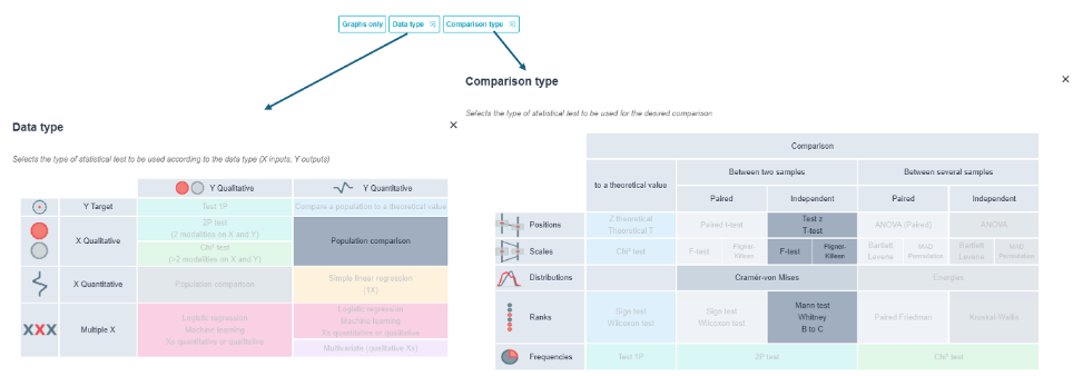
Conducting a test means answering the question, «Is there a difference between these situations?» or the question, «Can I conclude that these two situations are equivalent?»
These two questions cannot be answered using the same tests; that is why, when the situation allows, you will need to select the question by clicking on the appropriate badge.

2. The Tests Offered
2.1 To Show a Difference
| Family | Theoretical value | 2 samples | Several samples |
| Positions | Theoretical Z, Theoretical T | Z-test, t-test — Paired t-test | ANOVA — Paired ANOVA |
| Ladders | Chi-Square Test | F Test / Fligner-Killeen | Bartlett, Levene / MAD Permutation |
| Distributions | (based on descriptive statistics) | Cramér-von Mises | Energy |
| Ranks | Sign Test, Wilcoxon Test | Mann-Whitney Test, B to C | Kruskal-Wallis — Paired Friedman |
| Frequencies | Test 1P | Test 2P | Chi-Square Test |
When two tests are separated by a slash, the first one is parametric and the second nonparametric : The F-test and the Fligner-Killeen test address the same question, with the latter not assuming normality.
💡 Z or T? The Z-test assumes that the population standard deviation is known, which is rarely the case in practice. The T-test estimates it from the sample. When in doubt, use the T-test.
2.2 To Show an Equivalence
| Family | Theoretical value | 2 samples |
| Positions | TOST Two one-sided tests | TOST Two one-sided tests |
| Ladders | Scale Equivalence Variance Ratio | |
| Frequencies | Equivalence to a target proportionWilson score | Equivalence of Two ProportionsFarrington-Manning |
Ellistat automatically selects the appropriate tests based on the type of data you want to compare. No need to remember all the tests—Ellistat provides you with the complete results of the appropriate tests. For a continuous variable, it provides the tests for differences in location, scale, and dispersion! You can select just one of these categories.
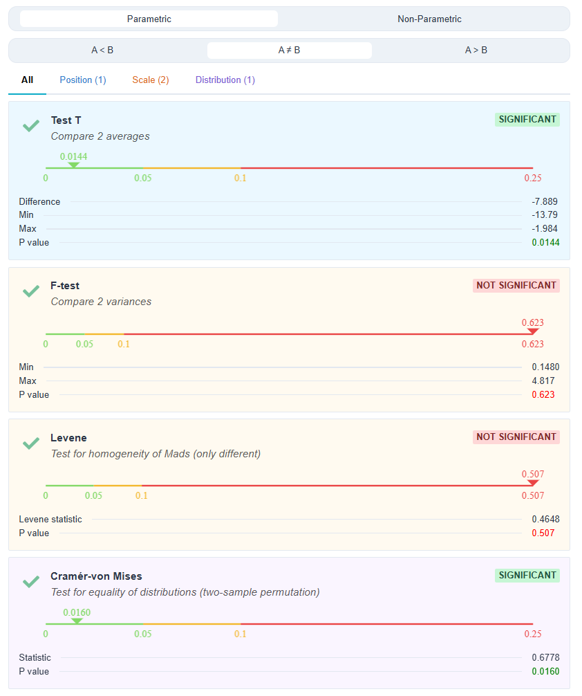
3. Parametric vs. Nonparametric Tests

Parametric tests assume a distribution, usually the normal distribution. They are more powerful when this assumption holds: given the same data, they detect smaller differences.
Nonparametric tests make no assumptions about the distribution. They are more robust but a little less sensitive.
- Normal distribution, no outliers: parametric ;
- Questionable laws, a small workforce, and extreme values: nonparametric.
The menu displays the two side by side precisely to make this choice clear.
Equivalence is available only in parametric : Switching to this option returns the selector to parametric mode. The non-parametric equivalent will be available in a future version.
4. Validity requirements, verified for you
This is a highlight of the menu, and one that’s often underutilized: Ellistat automatically checks the assumptions of the selected test and displays the verdict.
The three badges can be:
- The conditions have been met

- The conditions are being met despite a deviation from the ideal

- At least one condition is not met

| Condition | What Is Verified |
| Normal Law | Normality assumption accepted or rejected. For a paired test, it concerns the differencebetween samples, not on each sample. |
| Equivalence of Variances | The null hypothesis of equal variances is accepted or rejected. Some tests of the mean are sensitive to this. |
| Outliers | The presence or absence of outliers, which can, on their own, create or mask a difference. |
When a test has no condition to verify, Ellistat indicates this: «There is no hypothesis to verify for this test.» This is the case for nonparametric tests.
⚠️ A parametric test for which the assumptions are not met yields a p-value which does not have the advertised value. The natural response: switch to the non-parametric equivalent of the same line, or address the cause, remove a justified outlier, or transform the data.
💡 Never remove an outlier just because it’s inconvenient. An outlier is a information : data entry error, production issue, out-of-process part. It's better to understand it than to delete it.
5. Read the result
The results show the assumptions H0 and H1 stated explicitly for your case, the statistics of the test, the p-value, and the conclusion along with its result: Rejection of H0 or Non-rejection of H0.
The accompanying graph goes with the test: box-and-whisker plots for comparing means, and bar charts for proportions.
💡 Always look at the graph and the p-value together. The graph shows by how much and in what sense, the p-value indicates if that's to be believed. One without the other leaves half of the conclusion out.
6. Show an equivalence
A standard test aims to demonstrate a difference. He cannot prove the opposite: failing to find a difference is not the same as proving equality. Yet it is often equality that interests you: Is this new supplier as good as the old one? Does this faster adjustment yield the same measurement? Does this measuring method replace the previous one?
The selector Objective tips the test in that direction.

Only one new parameter: δ
δ is the equivalence limit : the tolerance below which the difference is of no concern to you. Its value is not based on statistics; it is a business decision—you are the one who decides that a deviation of two hundredths does not affect the part’s function.
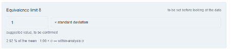
It is expressed as a unit of the characteristic, as % of the mean, as a multiple of the standard deviation, or as % of the tolerance interval—the most common formulation in industry. The other expressions are displayed below.
⚠️ δ is set before viewing the data. Choosing it after observing the discrepancy amounts to deciding on the conclusion, not testing it.
6.1 Reading is a visual process
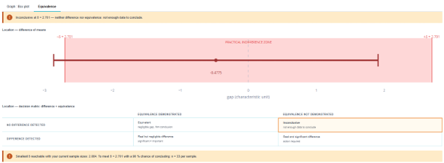
The tab Equivalence shows the confidence interval for the difference from the zone of indifference ±δ. Equivalence is demonstrated when the interval holds entirely in the area. No p-value is needed to see this.
6.2 The Decision Matrix
The two interpretations—difference and equivalence—overlap in four cases:

⚠️ The box Undecided is the one that the difference test alone hides. Without it, «not significant» is interpreted as «equal,» and that is incorrect.
6.3 How many pieces?

Two pieces of information replace the preliminary power calculation:
- the smallest provable δ with your current staff; ;
- the number of pieces what it would take to maintain the δ you have set.
6.4 Three Questions Instead of One
The alternative hypothesis line retains its role and is relabeled:

| Badge | Question |
 | Non-inferiority : A is not significantly worse than B |
 | Equivalence : A and B differ by no more than δ |
 | Non-superiority : A is not significantly better than B |
6.5 What does equivalence refer to?
Positions : means, for a single target or between two samples, whether matched or unmatched; ;
Ladders : variance ratio. The limit here is a **ratio R > 1**, the indifference region is `[1/R; R]`, and the graph is plotted on a logarithmic scale; ;
Frequencies : difference between two proportions or between a proportion and a target, in percentage points.
⚠️ Demonstrate equivalence of variances requires significantly higher production volumes than average runs—often several hundred pieces, whereas just a few dozen are sufficient for average runs. The exact number is displayed.
7. Several samples
A significant ANOVA or Kruskal-Wallis test indicates that «these groups are not all equal.» It does not say not which one is different.
To this end, Ellistat provides a conclusion in pairs, which compares the groups two by two.
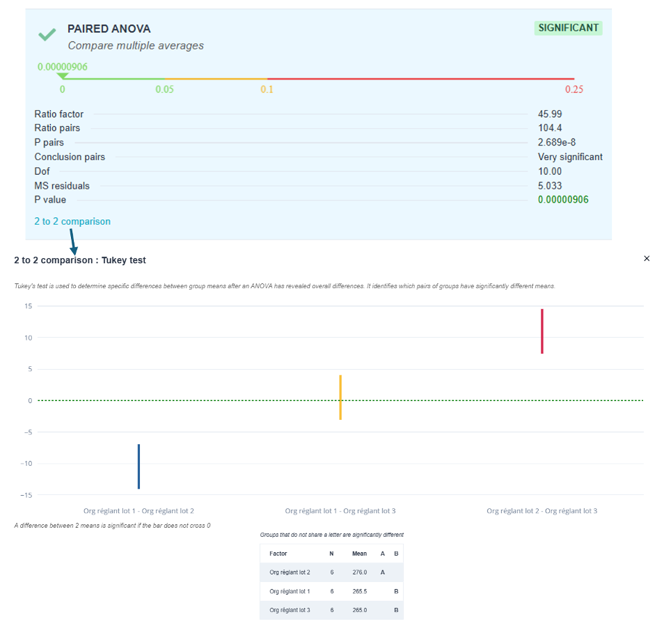
⚠️ Comparing all pairs increases the number of tests—and thus the number of false positives: with ten groups, we perform forty-five comparisons, and with a risk of 5 % for each, we find an average of two spurious differences. That is why you should use the provided pairwise comparison feature rather than performing t-tests manually one after another.
8. The Matching Trap
Data is paired when both series focus on the the same individuals : the same part before and after treatment, the same operator using two methods, the same part measured by two instruments.
The paired test eliminates between-subject variability and becomes much more powerful.
⚠️ Treating paired data as independent is the most common and costly mistake: the variability between samples masks the effect being sought, leading to the conclusion that «there is no difference» when in fact there is a clear difference. Conversely, classifying data sets as paired when they are not creates differences.
💡 The test indirectly reminds you of this: for a paired test, normality is checked on the difference. If Ellistat mentions the difference between samples, it means you're indeed dealing with a paired sample.
9. Analysis of variance when multiple X variables are selected and Y is quantitative
When multiple X variables are selected and Y is a quantitative variable, the nature of the question changes: it is no longer a matter of comparing two groups, but of determining which of the selected factors cause Y to vary. Ellistat then performs an analysis of variance on all the X variables.
The idea is to break down the observed variability in the Y variable: a portion attributable to each factor, and a residual portion that the model does not explain.
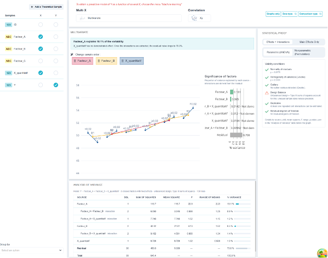
Here's what the page looks like:
- An analysis of variance table, with one row per factor: degrees of freedom, sum of squares, mean square, F-statistic, and p-value. A factor is considered significant when its p-value falls below the specified alpha level.
- The proportion of variability explained by each factor—which ranks the X variables relative to one another—and the residual proportion: the portion that the selected factors alone cannot explain.
- Related graphs: averages by method, box-and-whisker plots that show the direction and magnitude of the effect, whereas the p-value merely indicates its existence.
- For a factor with more than two levels, the pairwise comparison in §3.7 specifies which levels actually differ.
💡 Analyzing the Xs together is not the same as running a series of one-factor tests. Here, each effect is evaluated in the presence of the others: this avoids the accumulation of false-positive risks and distinguishes a factor that is truly influential from one that was influential only because of its association with another.
💡 Consider p-values and the proportion of variance explained together. With large sample sizes, a factor can be highly significant while explaining only a few percent of the variability: the effect is real, but the cause lies elsewhere.
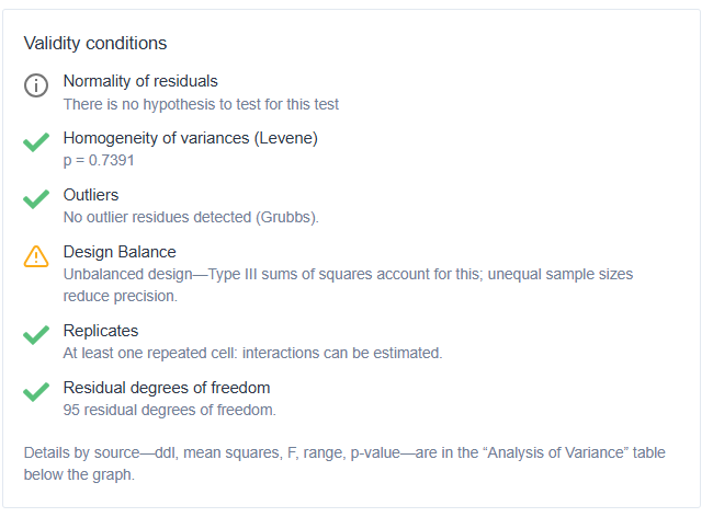
⚠️ The validity conditions in paragraph 4 also apply here, and they pertain to the model’s residuals: normality, homogeneity of variances across categories, and the absence of outliers. A single outlier can cause a factor to become significant.
⚠️ Analysis of variance establishes an association, not a cause: it indicates which factors are associated with variation in Y within the range actually covered by your data. To quantify the effects and their interactions, you need a design of experiments.
Table of Validity Conditions:
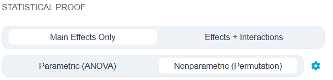
You can choose to include only the main effects or with the interactions. And also the calculation method Parametric or Nonparametric. The parametric method is the standard approach but requires the assumption of normality; the nonparametric method does not require this assumption and works by exchange. It is a time-consuming method. It applies only to tables with fewer than 1,000 rows. The results from the two methods are very similar, except in cases where the data is not normally distributed; in such cases, it is preferable to use the nonparametric approach.
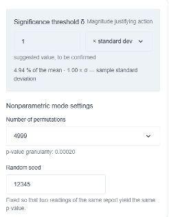
The gear icon allows you to select the following parameters: The smallest deviation worth considering as a deviation from the Y variable under study. This will be used in the decision matrix below. The number of permutations that results in the smallest change in the p-value. And the random seed: It is fixed, which ensures that the same results are always obtained on a given workstation.
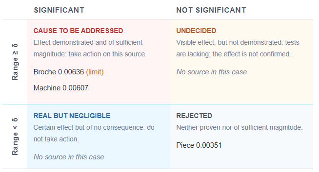
The decision matrix summarizes the status of all the factors studied based on their level of significance and their importance with respect to delta
⚠️ Note: In the case of a hierarchical structure, rather than analyzing interactions, it is preferable to use Generalized Analysis of Variance (ANOVA), which can be found in the «Sources of Variation» menu.»