


This is a reversal of the usual approach. Instead of drawing up a complete plan and then creating a model, we alternates : a few test runs, a model, the next test runs selected by the model, a better model, and so on. At each step, the software identifies the settings that yield the greatest improvement.
The tool is the Gaussian process : It predicts the answer and its uncertainty at any point in the domain. It is this uncertainty that allows us to make an informed choice about the next test; a point is of interest if it promises a good response, or if we don't know either way.
💡 It's the modern alternative to the simple, and the module handles it: same issues—costly processes, time-consuming tests, noisy measurements—but the Gaussian process takes advantage of all the information accumulated at each iteration, whereas the simplex considers only its most recent vertices.
1. Settle the case
The panel on the left, Study Parameters :
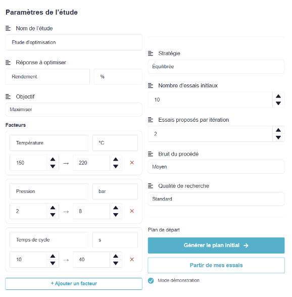
| Adjustment | Role |
| Study Name | Identifies the study, which is recorded in the project. |
| Response to be optimized | His name and his unit. |
| Objective | Maximize or Minimize the response. |
| Factors | A name, a minimum, and a maximum for each factor. «+ Add a factor,» and the trash can icon to remove one. |
| Trials of the Initial Plan (Audze-Eglais) | The number of initial trials, distributed evenly across the domain. |
| Suggested tests by iteration | The size of the lot offered in each round. |
| Optimization Strategy | Cautious, Balanced, Exploratory (see below). |
| Expected noise from the process | Low, Medium, High. |
| Research Quality | Quick, Standard, In-Depth. |
| Random seed | Makes the propositions reproducible. |
| Demo Mode (Process Simulator) | Practice the results to master the module. |
The button Generate the initial plan creates the first drafts. The factors are then locked : You can't change the field of study midway through without starting over—that's what Reset the study. The session is exported to JSON.
The Strategy Defines the "exploit/explore" trade-off:
- Cautious = Sticks close to areas that are already performing well and takes few risks. Ideal when testing is expensive
- Balanced = a balance between capitalizing on promising areas and exploring the unknown. The right default choice
- Exploratory = Also test areas of uncertainty to better understand the field. Useful at the beginning of a study.
Expected noise defines the range of noise that the model is allowed to estimate:
- Low = precise measurements, stable method: the model performs fine interpolation (noise ≤ ~5 % of the variance); ;
- Medium = general case, noise capped at ~25 %; ;
- High = highly variable measurements or processes: the model does not interpolate through noise (up to ~60 %).
Research Quality expands the pool of candidates considered for each proposal. In-Depth is recommended for more than 6 factors; it takes longer to calculate.
⚠️ The expected noise is the setting that has the greatest impact on the results, and it is reassessed as the study progresses. Declaring a process to be stable when it is not causes the model to interpret every measurement fluctuation as a real effect, leading subsequent tests down the wrong path. If the «high noise» warning appears in the diagnostic report, you must revisit this setting.
2. The Test Plan
This is the worksheet tab. A table, with one row per test:
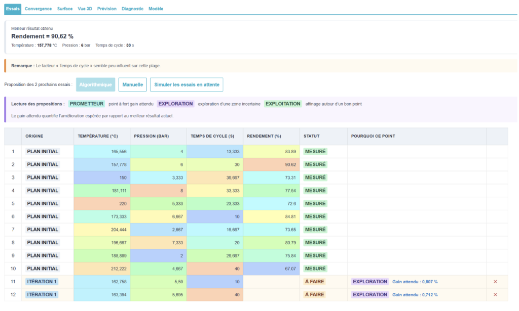
| Column | Contents |
| No. | The order of execution. |
| The Factors | The values to be applied. |
| The Answer | Don't miss out! after the test. |
| Status | Measured or To Do. |
| Origin | Initial Plan, BO it. n (proposed for the iteration n) or Manual. |
| Why this point? (model analysis) | Explanation of the proposal. |
The model adjusts based on at least 4 measured tests. Below that, the "Propose" button is disabled, and an explanation is provided. It also remains disabled as long as any proposed tests are awaiting results: a new batch is not proposed until the previous one has been processed.
The button Suggest the n upcoming trials Start the calculation. In demo mode, Simulate the results of pending tests fills in the answers.
Read the proposals = Each test provided has a label and a expected gain :
| Label | Meaning |
| Promising | The model potentially predicts better than the current best approach. This is the aspect that contributes most to the search for the optimal solution. |
| Operation | Close to the current best estimate: refines and improves the reliability of the optimum by reducing local uncertainty. |
| Exploration | An area that is still poorly understood, with a high degree of uncertainty. Provides information on unexplored regions and may reveal a better solution elsewhere. |
💡 The fact that two very similar options are offered is not a mistake. The module explicitly states this: the model focuses its efforts on an area deemed promising, to validate the measurement and separate the signal from the noise. This is the expected behavior for a noisy process, and it would be a mistake to «correct» these duplicates manually.
When the expected benefit of future trials becomes very low, a banner announces that Convergence is likely: We can either stop the study or continue it to confirm the findings.
3. Reading tabs
| Tab | What it shows |
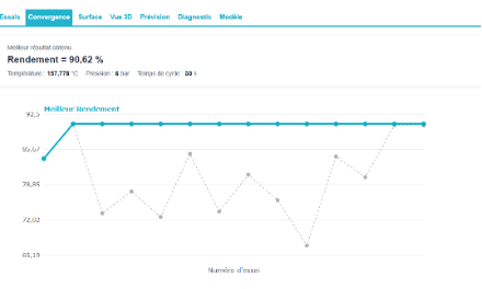
| Convergence | The best result achieved based on the test number. The curve that flattens out indicates convergence. At least two tests must be measured. |
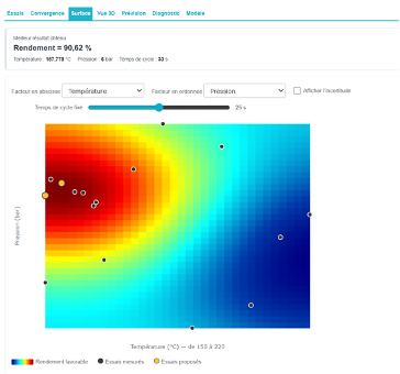
| Position of the points | The response surface predicted for two selected factors (with the others held constant), along with the experiments performed and the recommendations. A checkbox toggles the display to the’uncertainty instead of the answer. |
| 3D | Starting with two factors. Same for machine learning |
| 5D | Based on 4 factors. Same for machine learning |
| Forecast | The predicted answer at a specified point. Same as machine learning |
| Diagnostics (Reliability) | See Section 4.4. |
| Factors & Model | See Section 4.5. |
💡 The display of the’uncertainty The point map is the best decision-making tool in the entire module: it shows where the model has no information. A red zone of uncertainty at the edge of the domain alone explains why the proposals diverge there.
3.1 Convergence tab:
3.2 Surface Tab:
The black dots represent test results, and the brown dots represent proposed values
4. Assessment: Can I trust the model?
That is the question the tab literally asks, and it answers it with a leave-one-out cross-validation : Each trial is predicted as if it had never been done. This tests the model's actual ability to generalize, rather than its ability to revisit its own points.
An overall verdict:
- Generally Reliable Model,
- A model to be used with caution,
- Model is still somewhat unreliable
Then four indicators:
| Indicator | Reading |
| Predictive R² (Q²) | Prediction quality: good, average, or poor. |
| RMSE (LOO) | The standard prediction error, in the unit of the response. |
| MAE (LOO) | The mean absolute error. |
| Cover 95 % | The percentage of tests that fall within the reported range. |
Two charts are included: observed vs. predicted and residuals vs. predicted values with a 95% confidence interval of %, with each point labeled as "correctly predicted" or "incorrectly predicted.".
⚠️ The cover is the most important indicator and the one that is least often looked at. Below 95 %, the model underestimates his own uncertainty : Its intervals are too narrow, so its predictions are too confident. The module then recommends increasing the expected noise or adding more trials.
⚠️ With very few trials, the leave-one-out validation is itself not very robust—the module flags this. It should be reevaluated after a few iterations rather than taken at face value on the third trial.
5. Factors and Model
The tab displays the model itself: Matérn 5/2 Anisotropic Core, marginal log-likelihood, and the’estimated standard deviation of the noise, the measurement and process variability that the model accounts for.
Above all, it displays the indicative sensitivity of the model (ARD) : A factor with a short correlation length is one that, from the model's perspective, causes the response to vary significantly.
⚠️ The module is clear on this point, and it bears repeating: this sensitivity is an interpretation of the model, not a significance test or an analysis of variance. It identifies potential avenues; a dedicated statistical analysis confirms them.
Warnings appear depending on the status of the study: too few trials relative to the number of hyperparameters to be estimated, estimated noise is high or significant, and the correlation length is either at the lower limit (risk of overfitting) or at the upper limit (the model detects virtually no effect).